import Pkg
Pkg.activate(@__DIR__)
Pkg.instantiate()Homework 1: Simulation-Based Data Analysis
BEE 4850/5850, Fall 2024
You can find a Jupyter notebook, data, and a Julia 1.9.x environment in the homework’s Github repository. You should feel free to clone the repository and switch the notebook to another language, or to download the relevant data file(s) and solve the problems without using a notebook. In either of these cases, if you using a different environment, you will be responsible for setting up an appropriate package environment.
Regardless of your solution method, make sure to include your name and NetID on your solution PDF for submission to Gradescope.
Overview
Instructions
The goal of this homework assignment is to introduce you to simulation-based data analysis.
- Problem 1 asks you to explore whether a difference between data collected from two groups might be statistically meaningful or the result of noise. This problem repeats the analysis from Statistics Without The Agonizing Pain by John Rauser (which is a neat watch!).
- Problem 2 asks you to evaluate an interview method for finding the level of cheating on a test to determine whether cheating was relatively high or low. This problem was adapted from Bayesian Methods for Hackers.
- Problem 3 asks you to assess the quality of fit of a normal distribution to realizations from a Galton Board simulation.
- Problem 4 (graded only for graduate students) asks you to simulate outcomes from the Price Is Right Showcase game to identify a bidding strategy.
Load Environment
The following code loads the environment and makes sure all needed packages are installed. This should be at the start of most Julia scripts.
The following packages are included in the environment (to help you find other similar packages in other languages). The code below loads these packages for use in the subsequent notebook (the desired functionality for each package is commented next to the package).
using Random # random number generation and seed-setting
using DataFrames # tabular data structure
using CSVFiles # reads/writes .csv files
using Distributions # interface to work with probability distributions
using Plots # plotting library
using StatsBase # statistical quantities like mean, median, etc
using StatsPlots # some additional statistical plotting tools
Problems
Each problem in this assignment is worth 10 points.
Problem 1
The underlying question we would like to address is: what is the influence of drinking beer on the likelihood of being bitten by mosquitoes? There is a mechanistic reason why this might occur: mosquitoes are attracted by changes in body temperature and released CO2, and it might be that drinking beer induces these changes. We’ll analyze this question using (synthetic) data which separates an experimental population into two groups, one which drank beer and the other which drank only water.
First, we’ll load data for the number of bites reported by the participants who drank beer. This is in a comma-delimited file, data/bites.csv (which is grossly overkill for this assignment). Each row contains two columns: the group (beer and water) the person belonged to and the number of times that person was bitten.
In Julia, we can do this using CSVFiles.jl, which will read in the .csv file into a DataFrame, which is a typical data structure for tabular data (and equivalent to a Pandas DataFrame in Python or a dataframe in R).
data = DataFrame(load("data/bites.csv")) # load data into DataFrame

# print data variable (semi-colon suppresses echoed output in Julia, which in this case would duplicate the output)
@show data;
How can we tell if there’s a meaningful difference between the two groups? Naively, we might just look at the differences in group means.
Broadcasting
The subsetting operations in the below code use .==, which “broadcasts” the element-wise comparison operator == across every element. The decimal in front of == indicates that this should be used element-wise (every pair of elements compared for equality, returning a vector of true or false values); otherwise Julia would try to just check for vector equality (returning a single true or false value).
Broadcasting is a very specific feature of Julia, so this syntax would look different in a different programming language.
# split data into vectors of bites for each group
beer = data[data.group .== "beer", :bites]
water = data[data.group .== "water", :bites]

observed_difference = mean(beer) - mean(water)
@show observed_difference;
observed_difference = 4.37777777777778This tells us that, on average, the participants in the experiment who drank beer were bitten approximately 4.4 more times than the participants who drank water! Does that seem like a meaningful difference, or could it be the result of random chance?
We will use a simulation approach to address this question, as follows.
- Suppose someone is skeptical of the idea that drinking beer could result in a higher attraction to mosquitoes, and therefore more bites. To this skeptic, the two datasets are really just different samples from the same underlying population of people getting bitten by mosquitoes, rather than two different populations with different propensities for being bitten. This is the skeptic’s hypothesis, versus our hypothesis that drinking beer changes body temperature and CO2 release sufficiently to attract mosquitoes.
- If the skeptic’s hypothesis is true, then we can “shuffle” all of the measurements between the two datasets and re-compute the differences in the means. After repeating this procedure a large number of times, we would obtain a distribution of the differences in means under the assumption that the skeptic’s hypothesis is true.
- Comparing our experimentally-observed difference to this distribution, we can then evaluate the consistency of the skeptic’s hypothesis with the experimental results.
Why Do We Call This A Simulation-Based Approach?
This is a simulation-based approach because the “shuffling” is a non-parametric way of generating new samples from the underlying distribution (more on this later in the semester).
The alternative to this approach is to use a statistical test, such as a t-test, which may have other assumptions which may not be appropriate for this setting, particularly given the seemingly small sample sizes.
In this problem:
- Conduct the above procedure to generate 50,000 simulated datasets under the skeptic’s hypothesis.
- Plot a histogram of the results and add a dashed vertical line to show the experimental difference (if you are using Julia, feel free to look at the Making Plots with Julia tutorial on the class website).
- Draw conclusions about the plausibility of the skeptic’s hypothesis that there is no difference between groups. Feel free to use any quantitative or qualitative assessments of your simulations and the observed difference.
Problem 2
You are trying to detect if how prevalent cheating was on an exam. You are skeptical of the efficacy of just asking the students if they cheated. You are also concerned about privacy — your goal is not to punish individual students, but to see if there are systemic problems that need to be addressed. Someone proposes the following interview procedure, which the class agrees to participate in:
Each student flips a fair coin, with the results hidden from the interviewer. The student answers honestly if the coin comes up heads. Otherwise, if the coin comes up tails, the student flips the coin again, and answers “I did cheat” if heads, and “I did not cheat”, if tails.
We have a hypothesis that cheating was not prevalent, and the proportion of cheaters was no more than 5% of the class; in other words, we expect 5 “true” cheaters out of a class of 100 students. Our TA is more jaded and thinks that cheating was more rampant, and that 30% of the class cheated. The proposed interview procedure is noisy: the interviewer does not know if an admission means that the student cheated, or the result of a heads. However, it gives us a data-generating process that we can model and analyze for consistency with our hypothesis and that of the TA.
In this problem:
- Derive and code a simulation model for the above interview procedure given the “true” probability of cheating \(p\).
- Simulate your model (for a class of 100 students) 50,000 times under the your hypothesis and the TA’s hypothesis, and plot the two resulting datasets.
- If you received 31 “Yes, I cheated” responses while interviewing your class, what could you conclude? Feel free to use any qualitative or quantiative assessments to justify your conclusions.
- How useful do you think the interview procedure is to identify systemic teaching? What changes to the design might you make?
Problem 3 (10 points)
Suppose that we ask a class of students to walk individually from one end of a field to the other and count the number of steps that they take in order to cover the distance. More than likely, each student will get a somewhat different answer. After each student has paced off the field, we then make a histogram of the number of steps taken by the individual students. For a sufficiently large number of students, this histogram would resemble a normal distribution, due to the Central Limit Theorem.
A Galton board (named after Sir Francis Galton, a pioneering statistician1, shown below, is a physical device that demonstrates the Central Limit Theorem. A Galton board has rows of pins arranged in a triangular shape, with each row of pins offset horizontally relative to the rows above and below it. As illustrated in Figure 1, the top row has one pin, the second row has two pins, and so forth. If you’ve watched The Price is Right, you’ve seen this as “Plinko”.
1 And, notably, a leading eugenicist, which is unfortunately a recurring theme with leading early statisticians…)
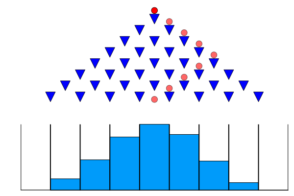
If a ball is dropped into the Galton board, it falls either to the right or the left when it bounces off the top pin. The ball then falls all the way to the bottom of the board, moving slightly to the right or left as it passes through each row of pins. Bins at the bottom of the board capture the ball and record its final position. If this experiment is repeated with many balls, the number of balls in each bin resembles a normal distribution, which is expected due to the Central Limit Theorem.
Your goal in this exercise is to explore how well a normal distribution fits the outcomes of repeated Galton Board trials as the number increases using quantile-quantile plots. Assessing the appropriateness of a probability model for a data set is a key part of exploratory analysis; we will return to this theme repeatedly. Or, to put it another way, it’s time for you to play Plinko!
In this problem:
- Write a function
galton_simwhich simulatesnGalton board trials (assume the board has 8 board rows, as in the image above) and returns a vector with the number of balls which fall into each bin. You can assume (for now) that the board is fair, e.g. that the probability of a left or right bounce is 0.5; you may want to make this probability a function parameter so you can change it later. - Run your simulation for a sample of 50 balls. Create a histogram of the results, with each bar corresponding to one bin. Make sure you use a random seed for reproducibility, and label your axes!
- Each Galton board trial can be represented as a realization from a binomial distribution. But as we noted above, by the Central Limit Theorem, the distribution of a large enough number of trials should be approximately normal. Use a quantile-quantile (Q-Q) plot to compare a fitted normal distribution with your simulation results. How well does a normal distribution fit the data?
- Repeat your simulation experiment with 250 trials and compare to a normal distribution. Does it describe the empirical distribution better?
- If the probability of a left bounce is 70%, what does this do to the fit of a normal distribution? What other distribution might you use if not a normal and why?
Problem 4
GRADED FOR 5850 STUDENTS ONLY
Your mastery of the Central Limit Theorem has led you to win your game of Plinko, and it’s time for the Showcases. This is the final round of an episode of The Price is Right, matching the two big winners from the episode. Each contestant is shown a “showcase” of prizes, which are usually some combination of a trip, a motor vehicle, some furniture, and maybe some other stuff. They then each have to make a bid on the retail price of the showcase. The rules are:
- an overbid is an automatic loss;
- the contest who gets closest to the retail price wins their showcase;
- if a contestant gets within \(\$250\) of the retail price and is closer than their opponent, they win both showcases.
Thanks to exhaustive statistics kept by game show fans, in Season 51 of The Price is Right showcase values had the following properties:
- median: $33,0481;
- lowest-value: $20,432
- highest-value: $72,409
In this problem:
- Write down a model which encodes the Showcase rules as a function of the showcase value and your bid. You can assume that your wagering is independent of your opponent.
- Select and fit a distribution to the above statistics (you have some freedom to pick a distribution, but make sure you justify it).
- Using 1,000 samples from your price distribution in your model, plot the expected winnings for bids from $20,000 through $72,000.
- Find the bid which maximizes your expected winnings. If you were playing The Price Is Right, is this the strategy you would adopt, or are there other considerations you would take into account which were not included in this model?