Model Complexity and Emulation


Lecture 21

April 29, 2024

Review of Model Selection

What Is The Goal of Model Selection?

Key Idea: Model selection consists of navigating the bias-variance tradeoff.

Bias and Variance

Model error (e.g. MSE) is a combination of irreducible error, bias, and variance.

  • Bias can come from under-dispersion (too little complexity) or neglected processes;
  • Variance can come from over-dispersion (too much complexity) or poor identifiability.

Cross-Validation

Cross-validation is the gold standard for predictive accuracy: how well does the fitted model predict out of sample data?

Cross-Validation

The problems:

  • Leave-one-out CV can be very computationally expensive!
  • We often don’t have a lot of data for calibration, so holding some back can be a problem.
  • How to divide data with spatial or temporal structure? This can be addressed by partitioning the data more cleverly (e.g. leaving out future observations), but makes the data problem worse.

Information Criteria

Approximate LOO-CV by computing fit on calibration/training data and “correcting” for expected overfitting.

Examples (differ in the parameter values used and correction factor(s)):

  • AIC
  • DIC
  • WAIC

Model Weighting

Information Criteria can be used to get averaging weights across a model set \(\mathcal{M} = \{M_1, \ldots, M_m\}\):

\[w_i = \frac{\exp(-\Delta_i/2)}{\sum_{m=1}^M \exp(-\Delta_m/2)}.\]

Bayesian LOO-CV: Advanced Methods

There are approximations to Leave-One-Out Cross-Validation which use importance sampling to avoid this, and these can be extended to time series.

See:

  • Vehtari et al. (2017) on approximations to LOO-CV;
  • Bürkner et al. (2020) on “leave-future-out” time series CV;
  • Yao et al. (2018) on modeling stacking for averaging.

Model Complexity

Parsimony as A Modeling Virtue

Parsimony (fewer model terms/components) can reduce the chance of overfitting and increased variance, all else being equal.

Model simplicity has another advantange: simpler models are less computationally expensive.

Computational Budgets

Computational Budgets

Source: Helgeson et al. (2021)

Benefits of Model Simplicity

  • More thorough representation of uncertainties
  • Can focus on “important” characteristics for problem at hand
  • Potential increase in generalizability

Computational Complexity

Source: Helgeson et al. (2021)

Downsides of Model Simplicity

  • Potential loss of salience
  • May miss important dynamics (creating bias)
  • Parameter/dynamical compensation can result in loss of interpretability

Simplicity Tradeoffs

Simple models can be epistemically and practically valuable.

But:

Need to carefully select which processes/parameters are included in the simplified representation, and at what resolution.

Emulation

Approximating Complex Models

Challenge: How do we simplify complex models to keep key dynamics but reduce computational expense?

Approximate (or emulate) the model response surface.

  1. Evaluate original model at an ensemble of points (design of experiment)
  2. Calibrate emulator against those points.
  3. Use emulator for UQ with MCMC or other methods.

Emulation of a 1-D Toy Model

Emulation of a Toy Model

Source: Haran et al. (2017)

Emulator of a Spatial (Ice Sheet) Model

Emulation of a Toy Model

Source: Haran et al. (2017)

Setting Up Emulation

  1. Select design points (design of experiment) and evaluate main model.
  2. Calibrate surrogate model to design inputs/outputs.

Design of Experiments

Important to strike a balance betwee:

  • Computational expense for model evaluation
  • Dense/expansive enough sample for training

Sampling Example

Code
# https://www.sfu.ca/~ssurjano/forretal08.html
# Forrester et al. (2008) Function
f(x) = (6 * x - 2)^2 * sin(12 * x - 4)

n_samples = 10
lower_bound = 0.0
upper_bound = 1.0

xs = lower_bound - 0.1:0.001:upper_bound + 0.1

xsmall = Surrogates.sample(4, lower_bound, upper_bound, SobolSample())
ysmall = f.(xsmall)
surrogate_small = Kriging(xsmall, ysmall, lower_bound, upper_bound)
xsobol = Surrogates.sample(n_samples, lower_bound, upper_bound, SobolSample())
ysobol = f.(xsobol)
surrogate_sobol = Kriging(xsobol, ysobol, lower_bound - 0.1, upper_bound + 0.1)

p1 = plot(; xlims=(lower_bound - 0.1, upper_bound + 0.1), legendfontsize=18, guidefontsize=18, tickfontsize=16, xlabel=L"$x$", ylabel=L"$f(x)$", size=(800, 500))
plot!(p1, xs, f.(xs), label="True Function", color=:red, linewidth=3)
scatter!(p1, xsobol, ysobol, color=:black, markersize=7, label="10 Samples")
plot!(p1, xs, surrogate_sobol.(xs), label = "Surrogate Function",
    ribbon = x -> std_error_at_point(surrogate_sobol, x), color=:black, alpha=0.3, linewidth=2)

p2 = plot(; xlims=(lower_bound - 0.1, upper_bound + 0.1), legendfontsize=18, guidefontsize=18, tickfontsize=16, xlabel=L"$x$", ylabel=L"$f(x)$", size=(800, 500))
plot!(p2, xs, f.(xs), label="True Function", color=:red, linewidth=3)
scatter!(p2, xsmall, ysmall, color=:darkorange, markersize=7, label="4 Samples")
plot!(p2, xs, surrogate_small.(xs), label = "Surrogate Function",
    ribbon = x -> std_error_at_point(surrogate_small, x), color=:darkorange, alpha=0.3, linewidth=2)

plot(p1, p2, size=(1200, 500), left_margin=5mm, bottom_margin=5mm)
Figure 1

Design of Experiments

Code
xrand = rand(Uniform(lower_bound, upper_bound), 10)
xsobol = Surrogates.sample(n_samples, lower_bound, upper_bound, SobolSample())
yrand = f.(xrand)
ysobol = f.(xsobol)

p = plot(; xlims=(lower_bound, upper_bound), legendfontsize=18, guidefontsize=18, tickfontsize=16, xlabel=L"$x$", ylabel=L"$f(x)$", size=(800, 500))
plot!(p, xs, f.(xs), label="True Function", color=:red, linewidth=3)
scatter!(p, xrand, yrand, color=:blue, markersize=7, label="Monte Carlo Sample")
scatter!(p, xsobol, ysobol, color=:black, markersize=7, label="Sobol (Low-Discrepancy) Sample")
Figure 2

Design of Experiments Example

Code
surrogate_rand = Kriging(xrand, yrand, lower_bound - 0.1, upper_bound + 0.1)

p1 = plot(; xlims=(lower_bound - 0.1, upper_bound + 0.1), legendfontsize=18, guidefontsize=18, tickfontsize=16, xlabel=L"$x$", ylabel=L"$f(x)$", size=(800, 500))
plot!(p1, xs, f.(xs), label="True Function", color=:red, linewidth=3)
scatter!(p1, xrand, yrand, color=:blue, markersize=7, label="Monte Carlo Sample")
plot!(p1, xs, surrogate_rand.(xs), label = "Surrogate Function",
    ribbon = x -> std_error_at_point(surrogate_rand, x), color=:blue, alpha=0.3, linewidth=2)

p2 = plot(; xlims=(lower_bound - 0.1, upper_bound + 0.1), legendfontsize=18, guidefontsize=18, tickfontsize=16, xlabel=L"$x$", ylabel=L"$f(x)$", size=(800, 500))
plot!(p2, xs, f.(xs), label="True Function", color=:red, linewidth=3)

scatter!(p2, xsobol, ysobol, color=:black, markersize=7, label="Sobol Sample")
plot!(p2, xs, surrogate_sobol.(xs), label = "Surrogate Function",
    ribbon = x -> std_error_at_point(surrogate_sobol, x), color=:black, alpha=0.3, linewidth=2)

plot(p1, p2, size=(1200, 500), left_margin=5mm, bottom_margin=5mm)
Figure 3

Emulating Models and Discrepancies

We can emulate model response functions \(f\) by defining the surrogate on a set of parameters, e.g.:

\[\hat{f}(p_1, p_2, \ldots, p_n) \approx f(p_1, p_2, \ldots, p_n; q_1, q_2, \ldots, q_m)\]

We can also emulate the discrepancy of the model if we are not comfortable writing down a parametric model.

Is Emulation Always The Right Choice?

Emulation of a Toy Model

Source: Lee et al. (2020)

Impacts of “Poor” Emulation

This error can have large knock-on effects for risk analysis:

Emulation of a Toy Model

Source: Lee et al. (2020)

Key Takeaways and Upcoming Schedule

Key Takeaways (Simplicity)

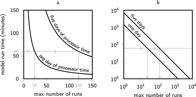
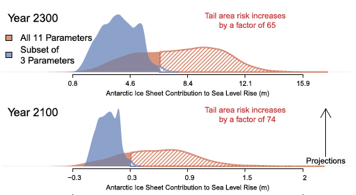
  • Model simplicity can be valuable for focusing on key dynamics and uncertainty representation.
  • Tradeoff between computational expense and fidelity of approximation.

Key Takeaways (Emulation)

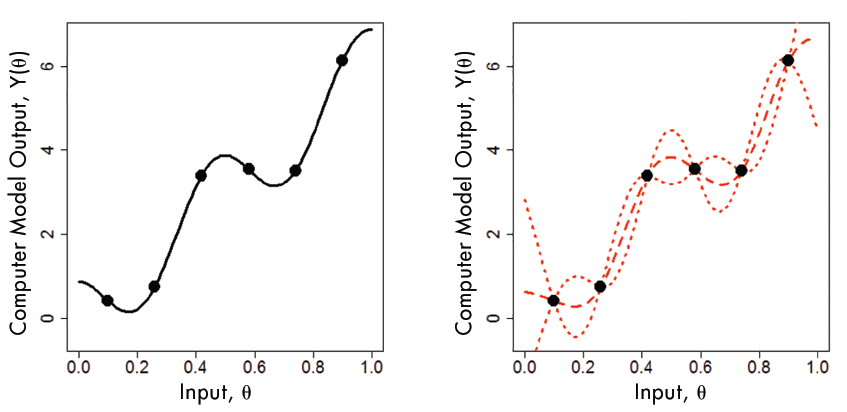
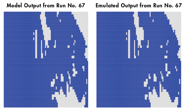
  • Emulation can “simplify” complex models by approximating response surfaces
  • Emulator methods have different pros and cons which can make them more or less important.
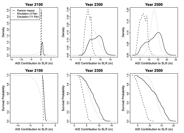
  • Emulator error can strongly influence resulting risk estimates.

Upcoming Schedule

Wednesday: Emulation Methods

Friday: HW4 due

Next Monday: Project Presentations, email slides by Saturday.

References

References

Bürkner, P.-C., Gabry, J., & Vehtari, A. (2020). Approximate leave-future-out cross-validation for bayesian time series models. J. Stat. Comput. Simul., (14), 2499–2523. https://doi.org/10.1080/00949655.2020.1783262
Haran, M., Chang, W., Keller, K., Nicholas, R., & Pollard, D. (2017). Statistics and the future of the antarctic ice sheet. Chance, 30(4), 37–44. https://doi.org/10.1080/09332480.2017.1406758
Helgeson, C., Srikrishnan, V., Keller, K., & Tuana, N. (2021). Why simpler computer simulation models can be epistemically better for informing decisions. Philos. Sci., 88(2), 213–233. https://doi.org/10.1086/711501
Lee, B. S., Haran, M., Fuller, R. W., Pollard, D., & Keller, K. (2020). A fast particle-based approach for calibrating a 3-D model of the antarctic ice sheet. Ann. Appl. Stat., 14(2), 605–634. https://doi.org/10.1214/19-AOAS1305
Vehtari, A., Gelman, A., & Gabry, J. (2017). Practical bayesian model evaluation using leave-one-out cross-validation and WAIC. Stat. Comput., 27(5), 1413–1432. https://doi.org/10.1007/s11222-016-9696-4
Yao, Y., Vehtari, A., Simpson, D., & Gelman, A. (2018). Using stacking to average Bayesian predictive distributions. arXiv [Stat.ME]. https://doi.org/10.1214/17-BA1091