Sampling from the posterior distribution \[p(\theta | \mathbf{y})\]
Sampling from the posterior predictive distribution \[p(\tilde{y} | \mathbf{y})\] by generating data.
Bayesian Computation and Monte Carlo
Bayesian computation involves Monte Carlo simulation from the posterior (predictive) distribution.
These samples can then be analyzed to identify estimators, credible intervals, etc.
Posterior Sampling
Trivial for extremely simple problems:
low-dimensional.
with “conjugate” priors (which make the posterior a closed-form distribution).
For example: normal likelihood, normal prior ⇒ normal posterior
A First Algorithm: Rejection Sampling
Idea:
Generate proposed samples from another distribution \(g(\theta)\) which covers the target \(p(\theta | \mathbf{y})\);
Accept those proposals based on the ratio of the two distributions.
Proposal Distribution for Rejection Sampling
Rejection Sampling Algorithm
Suppose \(p(\theta | \mathbf{y}) \leq M g(\theta)\) for some \(1 < M < \infty\).
Simulate \(u \sim \text{Unif}(0, 1)\).
Simulate a proposal \(\hat{\theta} \sim g(\theta)\).
If \(u < \frac{p(\hat{\theta} | \mathbf{y})}{Mg(\hat{\theta})},\) accept \(\hat{\theta}\). Otherwise reject.
Rejection Sampling Challenges
Probability of accepting a sample is \(1/M\), so the “tighter” the proposal distribution coverage the more efficient the sampler.
Need to be able to compute \(M\).
Finding a good proposal and computing \(M\) may not be easy (or possible) for complex posteriors!
How can we do better?
How Can We Do Better?
The fundamental problem with rejection sampling is that we don’t know the properties of the posterior. So we don’t know that we have the appropriate coverage. But…
What if we could construct an proposal/acceptance/rejection scheme that necessarily converged to the target distribution, even without a priori knowledge of its properties?
Markov Chain Basics
What Is A Markov Chain?
Consider a stochastic process \(\{X_t\}_{t \in \mathcal{T}}\), where
\(X_t \in \mathcal{S}\) is the state at time \(t\), and
\(\mathcal{T}\) is a time-index set (can be discrete or continuous)
\(\mathbb{P}(s_i \to s_j) = p_{ij}\).
Markov State Space
Markovian Property
This stochastic process is a Markov chain if it satisfies the Markovian (or memoryless) property: \[\begin{align*}
\mathbb{P}(X_{T+1} = s_i &| X_1=x_1, \ldots, X_T=x_T) = \\ &\qquad\mathbb{P}(X_{T+1} = s_i| X_T=x_T)
\end{align*}
\]
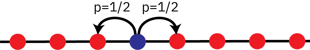
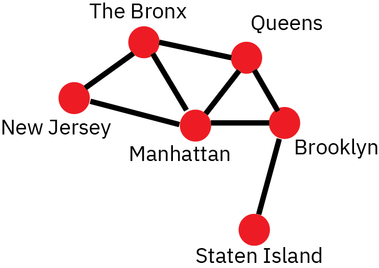
Example: “Drunkard’s Walk”
:img Random Walk, 80%
How can we model the unconditional probability \(\mathbb{P}(X_T = s_i)\)?
How about the conditional probability \(\mathbb{P}(X_T = s_i | X_{T-1} = x_{T-1})\)?
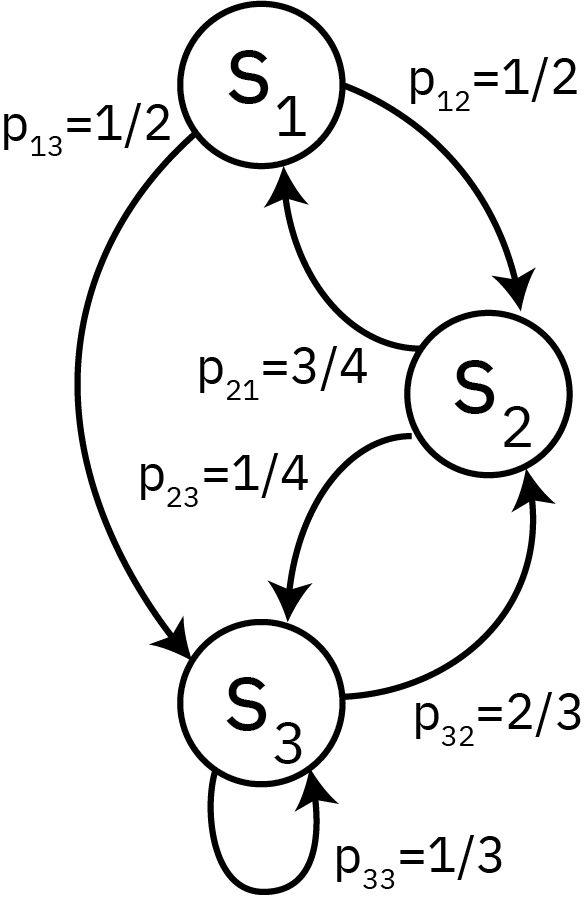
Example: Weather
Let’s look at a more interesting example. Suppose the weather can be foggy, sunny, or rainy.
Based on past experience, we know that:
There are never two sunny days in a row;
Even chance of two foggy or two rainy days in a row;
A sunny day occurs 1/4 of the time after a foggy or rainy day.
Aside: Higher Order Markov Chains
Suppose that today’s weather depends on the prior two days.
Can we write this as a Markov chain?
What are the states?
Weather Transition Matrix
We can summarize these probabilities in a transition matrix\(P\): \[
P =
\begin{array}{cc}
\begin{array}{ccc}
\phantom{i}\color{red}{F}\phantom{i} & \phantom{i}\color{red}{S}\phantom{i} & \phantom{i}\color{red}{R}\phantom{i}
\end{array}
\\
\begin{pmatrix}
1/2 & 1/4 & 1/4 \\
1/2 & 0 & 1/2 \\
1/4 & 1/4 & 1/2
\end{pmatrix}
&
\begin{array}{ccc}
\color{red}F \\ \color{red}S \\ \color{red}R
\end{array}
\end{array}
\]
Rows are the current state, columns are the next step, so \(\sum_i p_{ij} = 1\).
Weather Example: State Probabilities
Denote by \(\lambda^t\) a probability distribution over the states at time \(t\).
Figure 1: State probabilities for the weather examples.
Stationary Distributions
This stabilization always occurs when the probability distribution is an eigenvector of \(P\) with eigenvalue 1:
\[\pi = \pi P.\]
This is called an invariant or a stationary distribution.
What Markov Chains Have Stationary Distributions?
Not necessarily! The key is two properties:
Irreducible
Aperiodicity
Irreducibility
A Markov chain is irreducible if every state is accessible from every other state, e.g. for every pair of states \(s_i\) and \(s_j\) there is some \(k > 0\) such that \(P_{ij}^k > 0.\)
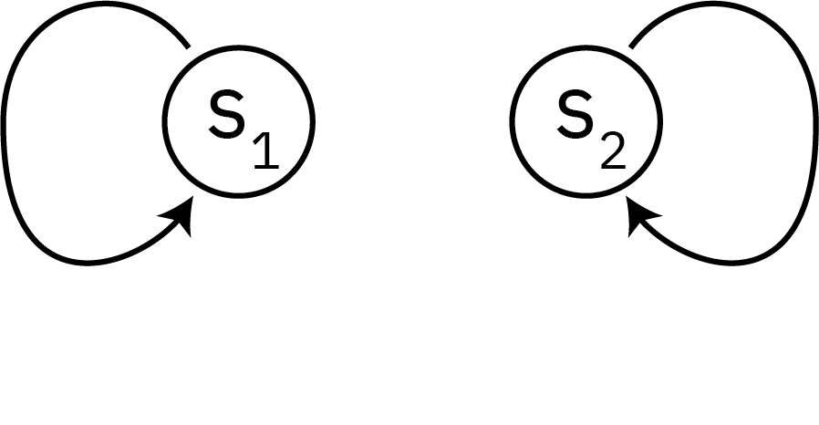
Reducible Markov Chain
Aperiodicity
The period of a state \(s_i\) is the greatest common divisor \(k\) of all \(t\) such that \(P^t_{ii} > 0\).
In other words, if a state \(s_i\) has period \(k\), all returns must occur after time steps which are multiples of \(k\).
A Markov chain is aperiodic if all states have period 1.
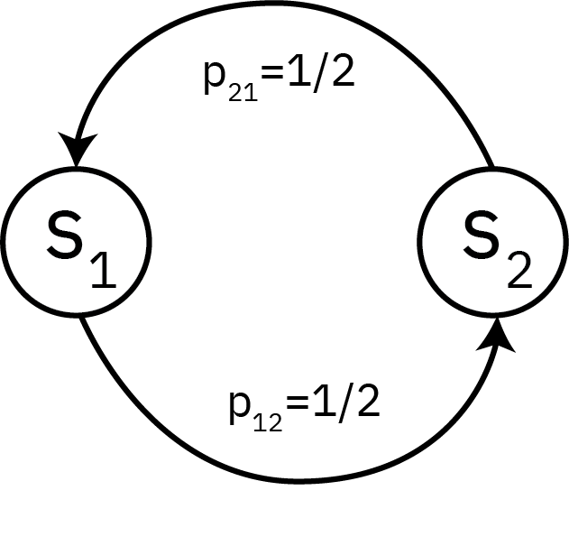
Periodic Markov Chain
Ergodicity
A Markov chain is ergodic if it is aperiodic and irreducible.
Ergodic Markov chains have a limiting distribution which is the limit of the time-evolution of the chain dynamics, e.g.\[\pi_j = \lim_{t \to \infty} \mathbb{P}(X_t = s_j).\]
Key: The limiting distribution limit is independent of the initial state probability.
Figure 2: Transient portion of the weather Markov chain.
Detailed Balance
The last important concept is detailed balance.
Let \(\{X_t\}\) be a Markov chain and let \(\pi\) be a probability distribution over the states. Then the chain is in detailed balance with respect to \(\pi\) if \[\pi_i P_{ij} = \pi_j P_{ji}.\]
Detailed balance implies reversibility: the chain’s dynamics are the same when viewed forwards or backwards in time.
The idea of our sampling algorithm (which we will discuss next time) is to construct an ergodic Markov chain from the detailed balance equation for the target distribution.
Detailed balance implies that the target distribution is the stationary distribution.
Ergodicity implies that this distribution is unique and can be obtained as the limiting distribution of the chain’s dynamics.
Idea of Sampling Algorithm
In other words:
Generate an appropriate Markov chain so that its stationary distribution of the target distribution \(\pi\);
Run its dynamics long enough to converge to the stationary distribution;
Use the resulting ensemble of states as Monte Carlo samples from \(\pi\) .
Sampling Algorithm
Any algorithm which follows this procedure is a Markov chain Monte Carlo algorithm.
Good news: These algorithms are designed to work quite generally, without (usually) having to worry about technical details like detailed balance and ergodicity.
Bad news: They can involve quite a bit of tuning for computational efficiency. Some algorithms or implementations are faster/adaptive to reduce this need.
Sampling Algorithm
Annoying news:
Convergence to the stationary distribution is only guaranteed asymptotically; evaluating if the chain has been run long enough requires lots of heuristics.
Due to Markovian property, samples are dependent, so smaller “effective sample size”.
Key Points and Upcoming Schedule
Key Points
Bayesian computation is difficult because we need to sample from effectively arbitrary distributions.
Markov chains provide a path forward if we can construct a chain satisfying detailed balance whose stationary distribution is the target distribution.
Then a post-convergence chain of samples is the same as a dependent Monte Carlo set of samples.