The Parametric Bootstrap


Lecture 12

March 11, 2024

Last Class

Sampling Distributions

The sampling distribution of a statistic captures the uncertainty associated with random samples.

Sampling Distribution

The Bootstrap Principle

Efron (1979) suggested combining estimation with simulation: the bootstrap.

Key idea: use the data to simulate a data-generating mechanism.

Baron von Munchhausen Pulling Himself By His Hair

Source: Wikipedia

Why Does The Bootstrap Work?

Let \(t_0\) the “true” value of a statistic, \(\hat{t}\) the estimate of the statistic from the sample, and \((\tilde{t}_i)\) the bootstrap estimates.

  • Variance: \(\text{Var}[\hat{t}] \approx \text{Var}[\tilde{t}]\)
  • Then the bootstrap error distribution approximates the sampling distribution \[(\tilde{t}_i - \hat{t}) \overset{\mathcal{D}}{\sim} \hat{t} - t_0\]

The Non-Parametric Bootstrap

The non-parametric bootstrap is the most “naive” approach to the bootstrap: resample-then-estimate.

Non-Parametric Bootstrap

Why Use The Bootstrap?

  • Do not need to rely on variance asymptotics;
  • Can obtain non-symmetric CIs.

Approaches to Bootstrapping Structured Data

  • Correlations: Transform to uncorrelated data (principal components, etc.), sample, transform back.
  • Time Series: Block bootstrap

Generalizing the Block Bootstrap

The rough transitions in the block bootstrap can really degrade estimator quality.

  • Improve transitions between blocks
  • Moving blocks (allow overlaps)

Sources of Non-Parametric Bootstrap Error

  1. Sampling error: error from using finitely many replications
  2. Statistical error: error in the bootstrap sampling distribution approximation

When To Use The Non-Parametric Bootstrap

  • Sample is representative of the data distribution
  • Doesn’t work well for extreme values!

The Parametric Bootstrap

The Parametric Bootstrap

  • Non-Parametric Bootstrap: Resample directly from the data.
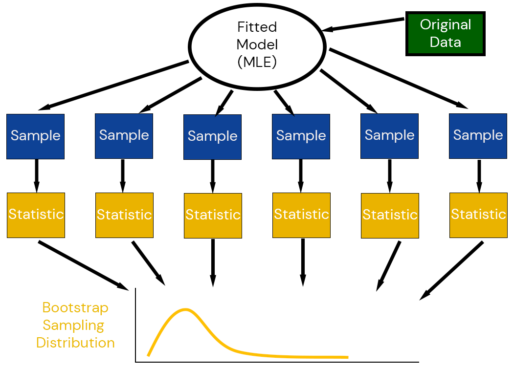
  • Parametric Bootstrap: Fit a model to the original data and simulate new samples, then calculate bootstrap estimates.

This lets us use additional information, such as a simulation or statistical model.

Parametric Bootstrap Scheme

The parametric bootstrap generates pseudodata using fitted model simulations.

Parametric Bootstrap

Benefits of the Parametric Bootstrap

  • Can quantify uncertainties in parameter values
  • Deals better with structured data (model accounts for structure)

Potential Drawbacks

  • New source of error: model specification
  • Misspecified models can completely distort estimates.

Example: 100-Year Return Periods

Detrended San Francisco Tide Gauge Data:

Code
# read in data and get annual maxima
function load_data(fname)
    date_format = DateFormat("yyyy-mm-dd HH:MM:SS")
    # This uses the DataFramesMeta.jl package, which makes it easy to string together commands to load and process data
    df = @chain fname begin
        CSV.read(DataFrame; header=false)
        rename("Column1" => "year", "Column2" => "month", "Column3" => "day", "Column4" => "hour", "Column5" => "gauge")
        # need to reformat the decimal date in the data file
        @transform :datetime = DateTime.(:year, :month, :day, :hour)
        # replace -99999 with missing
        @transform :gauge = ifelse.(abs.(:gauge) .>= 9999, missing, :gauge)
        select(:datetime, :gauge)
    end
    return df
end

dat = load_data("data/surge/h551.csv")

# detrend the data to remove the effects of sea-level rise and seasonal dynamics
ma_length = 366
ma_offset = Int(floor(ma_length/2))
moving_average(series,n) = [mean(@view series[i-n:i+n]) for i in n+1:length(series)-n]
dat_ma = DataFrame(datetime=dat.datetime[ma_offset+1:end-ma_offset], residual=dat.gauge[ma_offset+1:end-ma_offset] .- moving_average(dat.gauge, ma_offset))

# group data by year and compute the annual maxima
dat_ma = dropmissing(dat_ma) # drop missing data
dat_annmax = combine(dat_ma -> dat_ma[argmax(dat_ma.residual), :], groupby(transform(dat_ma, :datetime => x->year.(x)), :datetime_function))
delete!(dat_annmax, nrow(dat_annmax)) # delete 2023; haven't seen much of that year yet
rename!(dat_annmax, :datetime_function => :Year)
select!(dat_annmax, [:Year, :residual])
dat_annmax.residual = dat_annmax.residual / 1000 # convert to m

# make plots
p1 = plot(
    dat_annmax.Year,
    dat_annmax.residual;
    xlabel="Year",
    ylabel="Annual Max Tide (m)",
    label=false,
    marker=:circle,
    markersize=5,
    tickfontsize=16,
    guidefontsize=18
)
p2 = histogram(
    dat_annmax.residual,
    normalize=:pdf,
    orientation=:horizontal,
    label=:false,
    xlabel="PDF",
    ylabel="",
    yticks=[],
    tickfontsize=16,
    guidefontsize=18
)

l = @layout [a{0.7w} b{0.3w}]
plot(p1, p2; layout=l, link=:y, ylims=(1, 1.7), bottom_margin=10mm, left_margin=5mm)
plot!(size=(1000, 350))
Figure 1: Annual maxima surge data from the San Francisco, CA tide gauge.

Parametric Bootstrap Strategy

  1. Fit GEV Model
  2. Compute 0.99 Quantile
  3. Repeat \(N\) times:
    1. Resample Extreme Values from GEV
    2. Calculate 0.99 quantile.
  4. Compute Confidence Intervals

Parametric Bootstrap Results

Code
# function to fit GEV model for each data set
init_θ = [1.0, 1.0, 1.0]
gev_lik(θ) = -sum(logpdf(GeneralizedExtremeValue(θ[1], θ[2], θ[3]), dat_annmax.residual))

# get estimates from observations
rp_emp = quantile(dat_annmax.residual, 0.99)
θ_mle = Optim.optimize(gev_lik, init_θ).minimizer

p = histogram(dat_annmax.residual,  normalize=:pdf, xlabel="Annual Maximum Storm Tide (m)", ylabel="Probability Density", tickfontsize=16, guidefontsize=18, label=false, right_margin=5mm, bottom_margin=5mm, legendfontsize=18, left_margin=5mm)
plot!(p, GeneralizedExtremeValue(θ_mle[1], θ_mle[2], θ_mle[3]), linewidth=3, label="Parametric Model")
vline!(p, [rp_emp], color=:red, linewidth=3, linestyle=:dash, label="Empirical Return Level")
xlims!(p ,0, 2)
Figure 2: Fitted GEV Distribution

Adding Bootstrap Samples

Code
n_boot = 1000
boot_samp = rand(GeneralizedExtremeValue(θ_mle[1], θ_mle[2], θ_mle[3]), (nrow(dat_annmax), n_boot))
rp_boot = mapslices(col -> quantile(col, 0.99), boot_samp, dims=1)'

p = plot(GeneralizedExtremeValue(θ_mle[1], θ_mle[2], θ_mle[3]), linewidth=3, label="Parametric Model", xlabel="Annual Maximum Storm Tide (m)", ylabel="Probability Density", tickfontsize=16, guidefontsize=18, right_margin=5mm, bottom_margin=5mm, legendfontsize=18, left_margin=5mm)
vline!(p, [rp_emp], color=:red, linewidth=3, linestyle=:dash, label="Empirical Return Level")
xlims!(p ,0, 2)
scatter!(p, boot_samp[:, 1], zeros(nrow(dat_annmax)), color=:black, label="Bootstrap Replicates", markersize=5)
vline!(p, [rp_boot[1]], color=:grey, linewidth=2, label="Bootstrap Estimate")
Figure 3: Initial bootstrap sample

Bootstrap Confidence Interval

Code
p = histogram(rp_boot, xlabel="100-Year Return Period Estimate (m)", ylabel="Count", tickfontsize=16, guidefontsize=18, legendfontsize=18, label=false, right_margin=5mm, bottom_margin=5mm, left_margin=5mm)
vline!(p, [rp_emp], color=:red, linewidth=3, linestyle=:dash, label="Empirical Estimate")
q_boot = 2 * rp_emp .- quantile(rp_boot, [0.975, 0.025])
vspan!(p, q_boot, linecolor=:grey, fillcolor=:grey, alpha=0.3, fillalpha=0.3, label="95% CI")
Figure 4: Bootstrap histogram

When To Use The Parametric Bootstrap?

  • Reasonable to specify model (but uncertain about parameters/statistics);
  • Interested in statistics where model provides needed structure (e.g. extremes, dependent data);

Hybrid Bootstrap: Resampling Residuals

Residual Resampling Scheme

  1. Fit a trend/mechanistic model;
  2. Non-parametrically bootstrap residuals and refit model.

Example: Bootstrapping Sea-Level Rise

\[ \begin{gather*} H_t = F_t(\theta; T) + \varepsilon_t \\ \varepsilon_t \sim \mathcal{N}(0, \sigma) \end{gather*} \]

  1. Find MLE for \(\theta\);
  2. Resample residuals and add back;
  3. Refit model.

Residual Distribution from MLE Fit

Code
# load data files
slr_data = CSV.read("data/sealevel/CSIRO_Recons_gmsl_yr_2015.csv", DataFrame)
gmt_data = CSV.read("data/climate/HadCRUT.5.0.1.0.analysis.summary_series.global.annual.csv", DataFrame)
slr_data[:, :Time] = slr_data[:, :Time] .- 0.5; # remove 0.5 from Times
dat = leftjoin(slr_data, gmt_data, on="Time") # join data frames on time

# slr_model: function to simulate sea-level rise from global mean temperature based on the Rahmstorf (2007) model
function slr_model(α, T₀, H₀, temp_data)
    temp_effect = α .* (temp_data .- T₀)
    slr_predict = cumsum(temp_effect) .+ H₀
    return slr_predict
end

# split data structure into individual pieces
years = dat[:, 1]
sealevels = dat[:, 2]
temp = dat[:, 4]

# write function to calculate likelihood of residuals for given parameters
# parameters are a vector [α, T₀, H₀, σ]
function llik_normal(params, temp_data, slr_data)
    slr_out = slr_model(params[1], params[2], params[3], temp_data)
    resids = slr_out - slr_data
    return sum(logpdf.(Normal(0, params[4]), resids))
end

# set up lower and upper bounds for the parameters for the optimization
lbds = [0.0, -50.0, -200.0, 0.0]
ubds = [10.0, 1.0, 0.0, 20.0]
p0 = [5.0, -1.0, -100.0, 5.0]
p_mle = Optim.optimize(p -> -llik_normal(p, temp, sealevels), lbds, ubds, p0).minimizer

# compute residuals
slr_model_out = slr_model(p_mle[1], p_mle[2], p_mle[3], temp)
resids = slr_model_out - sealevels
histogram(resids, xlabel="Residual (mm)", ylabel="Count", legend=false, tickfontsize=16, guidefontsize=18, left_margin=5mm, bottom_margin=5mm)
Figure 5: Residuals from fitted SLR Model

Bootstrapped Realizations

Code
nboot = 1000
slr_boot = zeros(length(resids), nboot) # preallocate storage
for i = 1:nboot
    slr_boot[:, i] = slr_model_out + sample(resids, length(resids); replace=true)
end
p = plot(dat[:, 1], dat[:, 2], color=:black, linewidth=2, label="Observations", xlabel="Year", ylabel="Global Mean Sea Level (mm)", tickfontsize=16, guidefontsize=18, legendfontsize=18, left_margin=5mm, bottom_margin=5mm)
for idx in 1:10
    label = idx == 1 ? "Bootstrap Realizations" : false
    plot!(p, dat[:, 1], slr_boot[:, idx]; color=:grey, alpha=0.5, label=label, linewidth=1)
end
p
Figure 6: Bootstrap realizations from the SLR model

Bootstrap Estimates of SLR Temperature Sensitivity

Code
# fit model repeatedly
p_boot = mapslices(col -> Optim.optimize(p -> -llik_normal(p, temp, col), lbds, ubds, p0).minimizer, slr_boot, dims=1)

plt = histogram(p_boot[1, :], xlabel=L"$\alpha$ (mm/°C)", ylabel="Count", label=false, tickfontsize=16, guidefontsize=18, legendfontsize=18, left_margin=5mm, bottom_margin=10mm)
vline!(plt, [p_mle[1]], color=:red, linestyle=:dash, linewidth=3, label="Estimated Value")
q_boot = 2 * p_mle[1] .- quantile(p_boot[1, :], [0.975, 0.025])
vspan!(plt, q_boot, linecolor=:grey, fillcolor=:grey, alpha=0.3, fillalpha=0.3, label="95% CI")
plot!(plt, size=(1000, 400))
Figure 7: Bootstrap realizations from the SLR model

Interpreting the Bootstrap

What Does The Bootstrap Give Us?

The bootstrap gives us an estimate of the sampling distribution of a statistic or parameter.

We can use this for confidence intervals, statistical tests, bias correction, etc.

Bootstrap vs. Monte Carlo

Bootstrap “if I had a different sample (conditional on the bootstrap principle), what could I have inferred”?

Monte Carlo: Given specification of input uncertainty, what data could we generate?

Bootstrap Distribution and Monte Carlo

Could we use a bootstrap distribution for MC?

  • Sure, that’s just one specification of the data-generating process.
  • Nothing unique or particularly rigorous in using the bootstrap for this; substituting the bootstrap principle for other assumptions.

Bootstrap vs. Bayes

Bootstrap: “if I had a different sample (conditional on the bootstrap principle), what could I have inferred”?

Bayesian Inference: “what different parameters could have produced the observed data”?

Key Points and Upcoming Schedule

Key Points

  • Bootstrap Principle: Use the data as a proxy for the population.
  • Key: Bootstrap gives idea of sampling error in statistics (including model parameters)
  • Distribution of \(\tilde{t} - \hat{t}\) approximates distribution around estimate \(\hat{t} - t_0\).
  • Allows us to estimate uncertainty of estimates (confidence intervals, bias, etc).
  • Parametric bootstrap introduces model specification error

Bootstrap Variants

  • Resample Cases (Non-Parametric)
  • Resample Residuals (Semi-Parametric)
  • Simulate from Fitted Model (Parametric)

Which Bootstrap To Use?

  • Bias-Variance Tradeoff: Parametric Bootstrap has narrowest intervals, Resampling Cases widest (Exercise 8)
  • Depends on trust in model “correctness”:
    • Do we trust the model parameters to be “correct”?
    • Do we trust the shape of the regression model?
    • Do we trust the data-generating process?

Next Classes

Wednesday: Bayesian Computation and Markov chains

Next Week: Markov chain Monte Carlo

Assessments

  • Reading: Rahmstorf & Coumou (2011)
  • Exercise 8: Due Friday
  • Homework 3: Due 3/22

References

References

Efron, B. (1979). Bootstrap methods: Another look at the jackknife. Ann. Stat., 7, 1–26. https://doi.org/10.1214/aos/1176344552
Rahmstorf, S., & Coumou, D. (2011). Increase of extreme events in a warming world. Proceedings of the National Academy of Sciences, 108, 17905–17909. https://doi.org/10.1073/pnas.1101766108