Monte Carlo Simulation


Lecture 10

March 4, 2024

Previously In Class

Probability Models

  • Probability Models for Data-Generating Processes
  • Can be used for statistical models and simulation models (discrepancy)

What’s Next?

  • How do we:
    • Simulate from models/propagate uncertainty;
    • Go beyond MLE/MAP estimation for parameter values?
  • Model assessment/selection

Monte Carlo Simulation

Stochastic Simulation

Goal: Estimate \(\mathbb{E}_p\left[f(x)\right]\), \(x \sim p(x)\)

  • Standard approach: Compute \(\mathbb{E}_p\left[f(x)\right] = \int_X f(x)p(x)dx\)
  • Monte Carlo:
    • Sample \(x^1, x^2, \ldots, x^N \sim p(x)\)
    • Estimate \(\mathbb{E}_p\left[f(x)\right] \approx \sum_{n=1}^N f(x^n)\) / N

Monte Carlo Process Schematic

G a Probability Distribution b Random Samples a->b Sample c Model b->c Input d Outputs c->d Simulate

Goals of Monte Carlo

Monte Carlo is a broad method, which can be used to:

  1. Obtain probability distributions of outputs;
  2. Estimate deterministic quantities (Monte Carlo estimation).

MC Example: Finding \(\pi\)

How can we use MC to estimate \(\pi\)?

Hint: Think of \(\pi\) as an expected value…

MC Example: Finding \(\pi\)

Finding \(\pi\) by sampling random values from the unit square and computing the fraction in the unit circle. This is an example of Monte Carlo integration.

\[\frac{\text{Area of Circle}}{\text{Area of Square}} = \frac{\pi}{4}\]

Code
function circleShape(r)
    θ = LinRange(0, 2 * π, 500)
    r * sin.(θ), r * cos.(θ)
end

nsamp = 3000
unif = Uniform(-1, 1)
x = rand(unif, (nsamp, 2))
l = mapslices(v -> sum(v.^2), x, dims=2)
in_circ = l .< 1
pi_est = [4 * mean(in_circ[1:i]) for i in 1:nsamp]

plt1 = plot(
    1,
    xlim = (-1, 1),
    ylim = (-1, 1),
    legend = false,
    markersize = 4,
    framestyle = :origin,
    tickfontsize=16,
    grid=:false
    )
plt2 = plot(
    1,
    xlim = (1, nsamp),
    ylim = (3, 3.5),
    legend = :false,
    linewidth=3, 
    color=:black,
    tickfontsize=16,
    guidefontsize=16,
    xlabel="Iteration",
    ylabel="Estimate",
    right_margin=5mm
)
hline!(plt2, [π], color=:red, linestyle=:dash)
plt = plot(plt1, plt2, layout=Plots.grid(2, 1, heights=[2/3, 1/3]), size=(600, 500))

plot!(plt, circleShape(1), linecolor=:blue, lw=1, aspectratio=1, subplot=1)


mc_anim = @animate for i = 1:nsamp
    if l[i] < 1
        scatter!(plt[1], Tuple(x[i, :]), color=:blue, markershape=:x, subplot=1)
    else
        scatter!(plt[1], Tuple(x[i, :]), color=:red, markershape=:x, subplot=1)
    end
    push!(plt, 2, i, pi_est[i])
end every 100

gif(mc_anim, "figures/mc_pi.gif", fps=3)
[ Info: Saved animation to /Users/vs498/Teaching/BEE4850/sp24/slides/figures/mc_pi.gif
Figure 1: MCMC Estimation of pi

MC Example: Dice

What is the probability of rolling 4 dice for a total of 19?

Can simulate dice rolls and find the frequency of 19s among the samples.

Code
function dice_roll_repeated(n_trials, n_dice)
    dice_dist = DiscreteUniform(1, 6) 
    roll_results = zeros(n_trials)
    for i=1:n_trials
        roll_results[i] = sum(rand(dice_dist, n_dice))
    end
    return roll_results
end

nsamp = 10000
# roll four dice 10000 times
rolls = dice_roll_repeated(nsamp, 4) 

# calculate probability of 19
sum(rolls .== 19) / length(rolls)

# initialize storage for frequencies by sample length
avg_freq = zeros(length(rolls)) 
std_freq = zeros(length(rolls)) 

# compute average frequencies of 19
avg_freq[1] = (rolls[1] == 19)
count = 1
for i=2:length(rolls)
    avg_freq[i] = (avg_freq[i-1] * (i-1) + (rolls[i] == 19)) / i
    std_freq[i] = 1/sqrt(i-1) * std(rolls[1:i] .== 19)
end

plt = plot(
    1,
    xlim = (1, nsamp),
    ylim = (0, 0.1),
    legend = :false,
    tickfontsize=16,
    guidefontsize=16,
    xlabel="Iteration",
    ylabel="Estimate",
    right_margin=8mm,
    color=:black,
    linewidth=3,
    size=(600, 400)
)
hline!(plt, [0.0432], color="red", 
    linestyle=:dash) 

mc_anim = @animate for i = 1:nsamp
    push!(plt, 1, i, avg_freq[i])
end every 100

gif(mc_anim, "figures/mc_dice.gif", fps=10)
[ Info: Saved animation to /Users/vs498/Teaching/BEE4850/sp24/slides/figures/mc_dice.gif
Figure 2: MCMC Estimation of pi

Monte Carlo and Uncertainty Propagation

Monte Carlo simulation: propagate uncertainties from inputs through a model to outputs.

This is an example of uncertainty propagation: draw samples from some distribution, and run them through one or more models to find the (conditional) probability of outcomes of interest (for good or bad).

Uncertainty Propagation Flowchart

For example: What is the probability that a levee will be overtopped given climate and extreme sea-level uncertainty?

What Do We Need For MC?

  1. Simulation Model (Numerical/Statistical)
  2. Input Distributions

On Random Number Generators

Random number generators are not really random, only pseudorandom.

This is why setting a seed is important. But even that can go wrong…
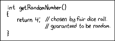
XKCD Cartoon 221: Random Number

Source: XKCD #221

Why Monte Carlo Works

Monte Carlo: Formal Approach

Formally: Monte Carlo estimation as the computation of the expected value of a random quantity \(Y\), \(\mu = \mathbb{E}[Y]\).

To do this, generate \(n\) independent and identically distributed values \(Y_1, \ldots, Y_n\). Then the sample estimate is

\[\tilde{\mu}_n = \frac{1}{n}\sum_{i=1}^n Y_i\]

The Law of Large Numbers

If

  1. \(Y\) is a random variable and its expectation exists and

  2. \(Y_1, \ldots, Y_n\) are independently and identically distributed

Then by the weak law of large numbers:

\[\lim_{n \to \infty} \mathbb{P}\left(\left|\tilde{\mu}_n - \mu\right| \leq \varepsilon \right) = 1\]

The Law of Large Numbers

In other words, eventually Monte Carlo estimates will get within an arbitrary error of the true expectation.

But how large is large enough?

Monte Carlo Sample Mean

The sample mean \(\tilde{\mu}_n = \frac{1}{n}\sum_{i=1}^n Y_i\) is itself a random variable.

With some assumptions (the mean of \(Y\) exists and \(Y\) has finite variance), the expected Monte Carlo sample mean \(\mathbb{E}[\tilde{\mu}_n]\) is

\[\frac{1}{n}\sum_{i=1}^n \mathbb{E}[Y_i] = \frac{1}{n} n \mu = \mu\]

Monte Carlo Error

We’d like to know more about the error of this estimate for a given sample size. The variance of this estimator is

\[\tilde{\sigma}_n^2 = \text{Var}\left(\tilde{\mu}_n\right) = \mathbb{E}\left((\tilde{\mu}_n - \mu)^2\right) = \frac{\sigma_Y^2}{n}\]

So as \(n\) increases, the standard error decreases:

\[\tilde{\sigma}_n = \frac{\sigma_Y}{\sqrt{n}}\]

Monte Carlo Error

In other words, if we want to decrease the Monte Carlo error by 10x, we need 100x additional samples. This is not an ideal method for high levels of accuracy.

Monte Carlo is an extremely bad method. It should only be used when all alternative methods are worse.

— Sokal, Monte Carlo Methods in Statistical Mechanics, 1996

But…often most alternatives are worse!

When Might We Want to Use Monte Carlo?

If you can compute your answers analytically or through quadrature, you probably should.

But for many “real” problems, this is either

  1. Not possible (or computationally intractable);
  2. Requires a lot of stylization and simplification.

Monte Carlo Confidence Intervals

Basic Idea: The Central Limit Theorem says that with enough samples, the errors are normally distributed:

\[\left\|\tilde{\mu}_n - \mu\right\| \to \mathcal{N}\left(0, \frac{\sigma_Y^2}{n}\right)\]

Monte Carlo Confidence Intervals

The \(\alpha\)-confidence interval is: \[\tilde{\mu}_n \pm \Phi^{-1}\left(1 - \frac{\alpha}{2}\right) \frac{\sigma_Y}{\sqrt{n}}\]

For example, the 95% confidence interval is \[\tilde{\mu}_n \pm 1.96 \frac{\sigma_Y}{\sqrt{n}}.\]

Implications of Monte Carlo Error

Converging at a rate of \(1/\sqrt{n}\) is not great. But:

  • All models are wrong, and so there always exists some irreducible model error.
  • We often need a lot of simulations. Do we have enough computational power?

Key Points and Upcoming Schedule

Key Points

  • Monte Carlo: estimate by simulating summary statistics
  • Instead of computing integrals, approximate through sample summaries
  • MC estimates are themselves random quantities
  • Confidence intervals obtained through Central Limit Theorem
  • \(\tilde{\mu}_n \to \mu\) at rate \(1/\sqrt{n}\): not great!

Next Classes

Wednesday: Monte Carlo Examples: Flood Risk and Climate Change

Next Week: The Bootstrap

Assessments

Exercise 7: Assigned, due Friday

Reading: Kale et al. (2021)

References

References

Kale, A., Kay, M., & Hullman, J. (2021). Visual reasoning strategies for effect size judgments and decisions. IEEE Trans. Vis. Comput. Graph., 27, 272–282. https://doi.org/10.1109/TVCG.2020.3030335