Exploratory Data Analysis, Correlations, and Autocorrelations
Lecture 05
February 5, 2024
Last Class(es)
Probability Models
Goal: Write down a probability model for the data-generating process for \(\mathbf{y}\).
- Direct statistical model, \[\mathbf{y} \sim \mathcal{D}(\theta).\]
- Model for the residuals of a numerical model, \[\mathbf{r} = \mathbf{y} - F(\mathbf{x}) \sim \mathcal{D}(\theta).\]
Model Fitting as Maximum Likelihood Estimation
We can interpret fitting a model (reducing error according to some loss or error metric) as maximizing the probability of observing our data from this data generating process.
Exploratory Data Analysis (EDA)
EDA: Assessing Model-Data Fit
Examples:
- Skewness
- Tails
- Clusters
- (Auto)correlations
Curve Fitting
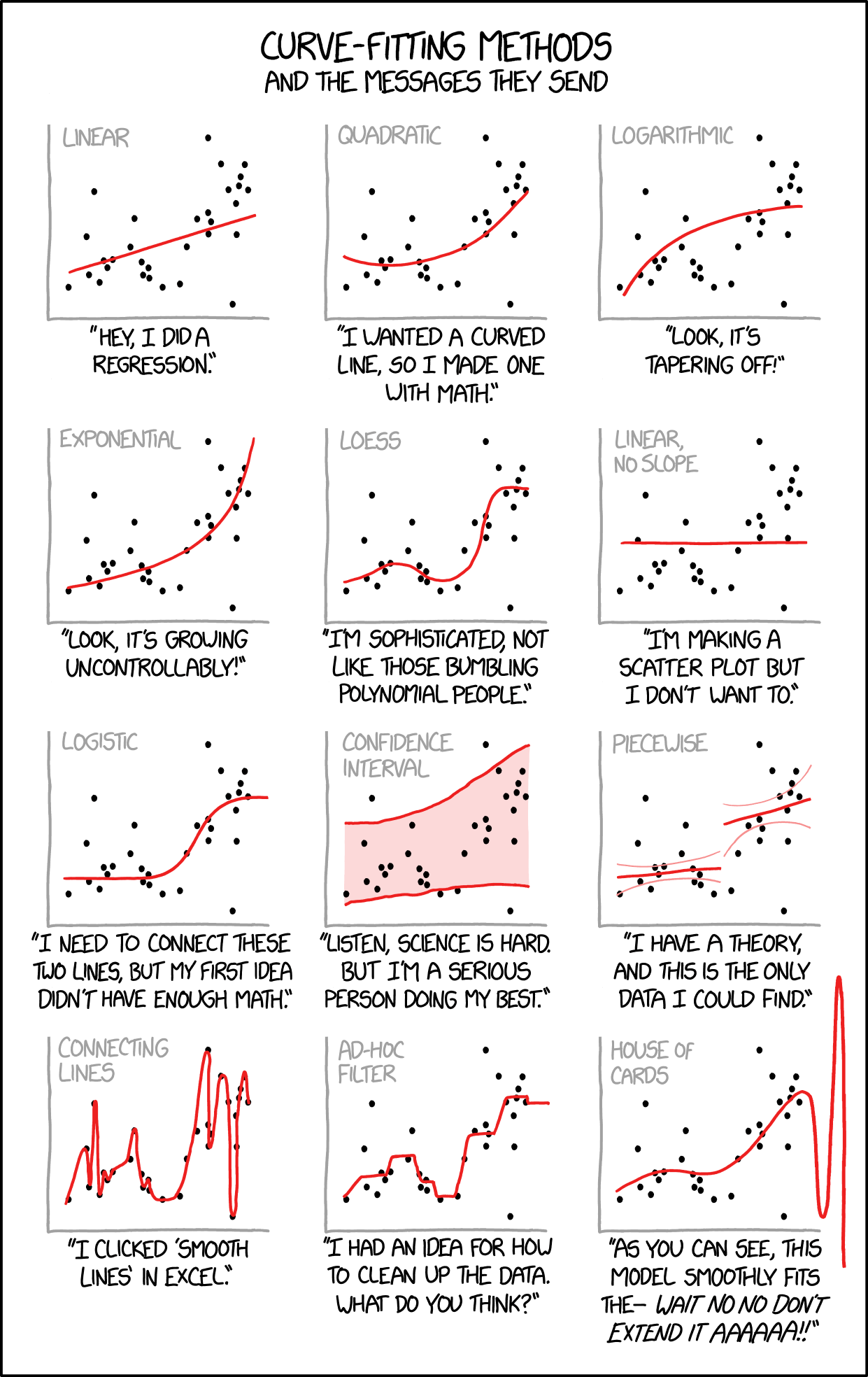
Source: XKCD #2048
Is EDA Ever Model-Free?
Some characterize EDA as model-free (versus “confirmatory” data analysis).
Is this right?
Visual Approaches to EDA
Make plots!
- Histograms
- Scatterplots/Pairs plots
- Quantile-Quantile Plots
Skew
Code
# specify regression model
f(x) = 2 + 2 * x
pred = rand(Uniform(0, 10), 20)
trend = f.(pred)

# generate normal residuals
normal_residuals = rand(Normal(0, 3), length(pred))
normal_obs = trend .+ normal_residuals

## generate skewed residuals
skewed_residuals = rand(SkewNormal(0, 3, 2), length(pred))
skewed_obs = trend .+ skewed_residuals

# make plots
# scatterplot of observations
p1 = plot(0:10, f.(0:10), color=:black, label="Trend Line", linewidth=2, guidefontsize=18, tickfontsize=16, legendfontsize=16) # trend line
scatter!(p1, pred, normal_obs, color=:orange, markershape=:circle, label="Normal Residuals")
scatter!(p1, pred, skewed_obs, color=:green, markershape=:square, label="Skewed Residuals")
xlabel!(p1, "Predictors")
ylabel!(p1, "Observations")
plot!(p1, size=(600, 450))

# densities of residual distributions
p2 = histogram(rand(Normal(0, 3), 1000), color=:orange, alpha=0.5, label="Normal Distribution", guidefontsize=18, tickfontsize=16, legendfontsize=16)
histogram!(p2, rand(SkewNormal(0, 3, 2), 1000), color=:green, alpha=0.5, label="SkewNormal Distribution")
xlabel!("Value")
ylabel!("Count")
plot!(p2, size=(600, 450))

display(p1)
display(p2)Fat Tails
Code
# generate normal residuals
normal_residuals = rand(Normal(0, 3), length(pred))
normal_obs = trend .+ normal_residuals

## generate fat-tailed residuals
cauchy_residuals = rand(Cauchy(0, 1), length(pred))
cauchy_obs = trend .+ cauchy_residuals

# make plots
# scatterplot of observations
p1 = plot(0:10, f.(0:10), color=:black, label="Trend Line", linewidth=2, guidefontsize=18, tickfontsize=16, legendfontsize=16) # trend line
scatter!(p1, pred, normal_obs, color=:orange, markershape=:circle, label="Normal Residuals")
scatter!(p1, pred, cauchy_obs, color=:green, markershape=:square, label="Fat-Tailed Residuals")
xlabel!(p1, "Predictors")
ylabel!(p1, "Observations")
plot!(p1, size=(600, 450))

# densities of residual distributions
p2 = histogram(rand(Normal(0, 3), 1000), color=:orange, alpha=0.5, label="Normal Distribution", guidefontsize=18, tickfontsize=16, legendfontsize=16)
histogram!(p2, rand(Cauchy(0, 1), 1000), color=:green, alpha=0.5, label="Cauchy Distribution")
xlabel!("Value")
ylabel!("Count")
plot!(p2, size=(600, 450))
xlims!(-20, 20)

display(p1)
display(p2)Quantile-Quantile (Q-Q) Plots
Particularly with small sample sizes, just staring at data can be unhelpful.
Q-Q plots are useful for checking goodness of fit of a proposed distribution.
Q-Q Plot Example
Code
## generate fat-tailed residuals
cauchy_samps = rand(Cauchy(0, 1), 20)

# make plots
# scatterplot of observations
p1 = plot(Normal(0, 2), linewidth=3, color=:green, label="Normal Distribution", yaxis=false, tickfontsize=16, guidefontsize=18, legendfontsize=18)
plot!(p1, Cauchy(0, 1), linewidth=3, color=:orange, linestyle=:dash, label="Cauchy Distribution")
xlims!(p1, (-10, 10))
xlabel!("Value")
plot!(p1, size=(500, 450))

# densities of residual distributions
p2 = qqplot(Normal, cauchy_samps, tickfontsize=16, guidefontsize=18, linewidth=3, markersize=6)
xlabel!(p2, "Theoretical Quantiles")
ylabel!(p2, "Empirical Quantiles")
plot!(p2, size=(500, 450))

display(p1)
display(p2)Predictive Checks
How well do projections match data (Gelman, 2004)?
Can be quantitative or qualitative.
Predictive Check: EBM Example
Code
# set number of sampled simulations
n_samples = 1000
residuals = rand(Normal(0, θ[end]), (n_samples, length(temp_obs)))
model_out = ebm_wrap(θ[1:end-1])
# this uses broadcasting to "sweep" the model simulation across the sampled residual matrix
model_sim = residuals .+ model_out' # need to transpose the model output vector due to how Julia treats vector dimensions

q_90 = mapslices(col -> quantile(col, [0.05, 0.95]), model_sim,; dims=1) # compute 90% prediction interval

plot(hind_years, model_out, color=:red, linewidth=3, label="Model Simulation", ribbon=(model_out .- q_90[1, :], q_90[2, :] .- model_out), fillalpha=0.3, xlabel="Year", ylabel="Temperature anomaly (°C)", guidefontsize=18, tickfontsize=16, legendfontsize=16, bottom_margin=5mm, left_margin=5mm)
scatter!(hind_years, temp_obs, color=:black, label="Data")
ylims!(-0.5, 1.2)Predictive Checks
Can also do predictive checks with summary statistics:
- Return periods
- Maximum/minimum values
- Predictions for out-of-sample data
Correlation and Auto-Correlation
What Is Correlation?
Correlation refers to whether two variables increase or decrease simultaneously.
Typically measured with Pearson’s coefficient:
\[r = \frac{\text{Cov}(X, Y)}{\sigma_X \sigma_Y} \in (-1, 1)\]
Correlation Examples
Code
# sample 1000 independent variables from a given normal distribution
sample_independent = rand(Normal(0, 1), (2, 1000))
p1 = scatter(sample_independent[1, :], sample_independent[2, :], label=:false, title="Independent Variables", tickfontsize=14, titlefontsize=18, guidefontsize=18)
xlabel!(p1, L"$x_1$")
ylabel!(p1, L"$x_2$")
plot!(p1, size=(400, 500))

# sample 1000 correlated variables, with r=0.7
sample_correlated = rand(MvNormal([0; 0], [1 0.7; 0.7 1]), 1000)
p2 = scatter(sample_correlated[1, :], sample_correlated[2, :], label=:false, title=L"Correlated ($r=0.7$)", tickfontsize=14, titlefontsize=18, guidefontsize=18)
xlabel!(p2, L"$x_1$")
ylabel!(p2, L"$x_2$")
plot!(p2, size=(400, 500))

# sample 1000 anti-correlated variables, with r=-0.7
sample_anticorrelated = rand(MvNormal([0; 0], [1 -0.7; -0.7 1]), 1000)
p3 = scatter(sample_anticorrelated[1, :], sample_anticorrelated[2, :], label=:false, title=L"Anticorrelated ($r=-0.7$)", tickfontsize=14, titlefontsize=18, guidefontsize=18)
xlabel!(p3, L"$x_1$")
ylabel!(p3, L"$x_2$")
plot!(p3, size=(400, 500))

display(p1)
display(p2)
display(p3)Correlation vs. Causation
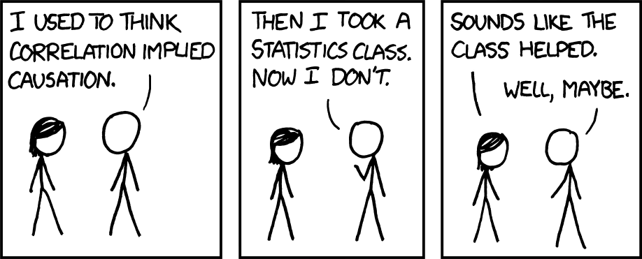
XKCD 552
Source: XKCD #552
“Correlation Does Not Imply Causation”
- Data can be correlated randomly (a spurious correlation)
- Data can be correlated due to a mutual causal factor
Spurious Correlations

Spurious Correlation Example
Source: Spurious Correlations #7602
Correlated Data Likelihood
- Marginal distributions normal: use a Multivariate Normal distribution
- Otherwise: Use copulas to “glue” marginal distributions together.
Autocorrelation
An important concept for time series is autocorrelation between \(y_t\) and \(y_{t-1}\).
Code
# sample independent series from a given normal distribution
sample_independent = rand(Normal(0, 1), 50)
p1 = plot(sample_independent, linewidth=3, ylabel=L"$y$", xlabel=L"$t$", title="Independent Series", guidefontsize=18, legend=:false, tickfontsize=16, titlefontsize=18)
plot!(p1, size=(500, 300))

# sample an autocorrelated series
sample_ar = zeros(50)
sample_ar[1] = rand(Normal(0, 1 / sqrt(1-0.6^2)))
for i = 2:50
    sample_ar[i] = 0.6 * sample_ar[i-1] + rand(Normal(0, 1))
end
p2 = plot(sample_ar, linewidth=3, ylabel=L"$y$", xlabel=L"$t$", title="Autocorrelated Series", guidefontsize=18, legend=:false, tickfontsize=16, titlefontsize=18)
plot!(p2, size=(500, 300))

display(p1)
display(p2)Lagged Regression
Code
# independent samples
dat = DataFrame(Y=sample_independent[2:end], X=sample_independent[1:end-1])
fit = lm(@formula(Y~X), dat)
pred = predict(fit,dat)
p1 = scatter(sample_independent[1:end-1], sample_independent[2:end], label=:false, title="Independent Variables: r=$(round(coef(fit)[2], digits=2))", tickfontsize=16, titlefontsize=18, guidefontsize=18)
plot!(p1, dat.X, pred, linewidth=2, label=:false)
ylabel!(p1, L"$y_t$")
xlabel!(p1, L"$y_{t-1}$")
plot!(p1, size=(600, 500))

# autocorrelated
dat = DataFrame(Y=sample_ar[2:end], X=sample_ar[1:end-1])
fit = lm(@formula(Y~X), dat)
pred = predict(fit,dat)
p2 = scatter(sample_ar[1:end-1], sample_ar[2:end], label=:false, title="Autocorrelated Variables: r=$(round(coef(fit)[2], digits=2))", tickfontsize=16, titlefontsize=18, guidefontsize=18)
plot!(p2, dat.X, pred, linewidth=2, label=:false)
ylabel!(p2, L"$y_t$")
xlabel!(p2, L"$y_{t-1}$")
plot!(p2, size=(600, 500))

display(p1)
display(p2)Autocorrelation Function
Many modern programming languages have autocorrelation functions (e.g. StatsBase.autocor() in Julia) which calculates the autocorrelation at varying lags.
Autocorrelation Function
But the autocorrelation function just computes the autocorrelations at every lag. Why is this a modeling problem?
Partial Autocorrelation Function
This is solved by using the partial autocorrelation function (e.g. StatsBase.pacf()):
Autoregressive Models
An autoregressive-with-lag-\(p\) (AR(\(p\))) model: \[y_t = \sum_{i=1}^{p} \rho_i y_{t-i} + \varepsilon_t\]
Example: An AR(1) model: \[ \begin{gather*} y_t = \rho y_{t-1} + \varepsilon_t \\ \varepsilon_t \sim \mathcal{N}(0, \sigma) \end{gather*} \]
AR(1) Likelihood
There are two ways to write down an AR(1) likelihood.
- “Whiten” the series:
\[ \begin{gather*} \varepsilon_t = y_t - y_{t-1} \sim \mathcal{N}(0, \sigma)\\ y_1 \sim \mathcal{N}\left(0, \frac{\sigma}{\sqrt{1-\rho^2}}\right) \end{gather*} \]
AR(1) Likelihood
- Joint likelihood:
\[ \mathbf{y} \sim \mathcal{N}(\mathbf{0}, \Sigma) \qquad \Sigma = \begin{pmatrix}\frac{\sigma^2}{1-\rho^2} & \rho & \rho^2 & \ldots & \rho^{T-1} \\ \rho & \frac{\sigma^2}{1-\rho^2} & \rho & \ldots & \rho^{T-2} \\ \vdots & \vdots & \vdots & \ddots & \vdots \\ \rho^{T-1} & \rho^{T-2} & \rho^{T-3} & \ldots & \frac{\sigma^2}{1-\rho^2} \end{pmatrix} \]
Model-Data Discrepancy
Model-Data Discrepancy
Model-data discrepancy: systematic disagreements between model and the modeled system state (Brynjarsdóttir & O’Hagan, 2014).
Let \(F(\mathbf{x}; \mathbf{\theta})\) be the simulation model:
- \(\mathbf{x}\) are the “control variables”;
- \(\mathbf{\theta}\) are the “calibration variables”.
Model-Data Discrepancy
If \(\mathbf{y}\) are the “observations,”” we can model these as: \[\mathbf{y} = z(\mathbf{x}) + \mathbf{\varepsilon},\] where
- \(z(\mathbf{x})\) is the “true” system state at control variable \(\mathbf{x}\);
- \(\mathbf{\varepsilon}\) are observation errors.
Model-Data Discrepancy
Then the discrepancy \(\zeta\) between the simulation and the modeled system is: \[\zeta(\mathbf{x}; \mathbf{\theta}) = z(\mathbf{x}) - F(\mathbf{x}; \mathbf{\theta}).\]
Then observations can be written as:
\[\mathbf{y} = F(\mathbf{x}; \mathbf{\theta}) + \zeta(\mathbf{x}; \mathbf{\theta}) + \mathbf{\varepsilon}.\]
Simple Discrepancy Example
Common to model observation errors as normally-distributed: \(\varepsilon_t \sim \mathcal{N}(0, \omega)\)
If the discrepancy is also i.i.d. normal: \(\zeta_t \sim \mathcal{N}(0, \sigma)\).
Residuals: \[\zeta_t + \varepsilon_t \sim \mathcal{N}(0, \sqrt{\omega^2 + \sigma^2})\]
Complex Discrepancy Example
Now suppose the discrepancy is AR(1).
\[\begin{gather*} \mathbf{\zeta} + \mathbf{\varepsilon} \sim \mathcal{N}(\mathbf{0}, \Sigma) \\ \Sigma = \begin{pmatrix}\frac{\sigma^2}{1-\rho^2} + {\color{red}\omega^2} & \rho & \rho^2 & \ldots & \rho^{T-1} \\ \rho & \frac{\sigma^2}{1-\rho^2} + {\color{red}\omega^2} & \rho & \ldots & \rho^{T-2} \\ \vdots & \vdots & \vdots & \ddots & \vdots \\ \rho^{T-1} & \rho^{T-2} & \rho^{T-3} & \ldots & \frac{\sigma^2}{1-\rho^2} + {\color{red}\omega^2} \end{pmatrix} \end{gather*} \]
Fitting Discrepancies
In many cases, separating discrepancy from observation error is tricky without prior information about variances.
Example: \[\zeta_t + \varepsilon_t \sim \mathcal{N}(0, \sqrt{\omega^2 + \sigma^2})\]
Not being able to separate \(\omega\) from \(\sigma\) is a problem called non-identifiability.
Discrepancies and Machine Learning
Can use machine learning models to “emulate” complex discrepancies and error structures.
More on ML as an emulation/error tool later in the semester.
Key Points and Upcoming Schedule
Key Points: EDA
- EDA helps identify a good or bad probability model;
- No black-box workflow: make plots, compare samples from proposed model to data, try to be skeptical
Key Points: Correlation
- Check for correlations, but think mechanistically.
- Use partial autocorrelation functions to find autoregressive model orders.
Key Points: Discrepancy
- Separate out “model bias” from observation errors.
- Often neglected: can be hard to fit without prior information on parameters.
- Use provided observation error variances when available to avoid non-identifiability.
Next Class(es)
Wednesday: Bayesian Statistics and Prior Information
Assessments
Friday: Exercise 1 due by 9pm.
HW2 assigned this week (will announce on Ed), due 2/23 by 9pm.
References
References
Brynjarsdóttir, J., & O’Hagan, A. (2014). Learning about physical parameters: the importance of model discrepancy. Inverse Problems, 30, 114007. https://doi.org/10.1088/0266-5611/30/11/114007
Gelman, A. (2004). Exploratory Data Analysis for Complex Models. J. Comput. Graph. Stat., 13, 755–779. https://doi.org/10.1198/106186004X11435