Uncertainty and Probability Review

---

Lecture 02

January 24, 2024

Overview

• Last Class
• Uncertainty
• Probability Distributions
• Uncertainty and Probability
• Recap

Last Class

Modes of Data Analysis

Workflow/Course Organization

Questions?

Text: VSRIKRISH to 22333

URL: https://pollev.com/vsrikrish

See Results

Uncertainty

What Is Uncertainty?

…A departure from the (unachievable) ideal of complete determinism…

— Walker et al. (2003)

Types of Uncertainty

• Aleatoric uncertainty: Uncertainties due to randomness/stochasticity;
• Epistemic uncertainty: Uncertainties due to lack of knowledge.

Data-Relevant Uncertainty Taxonomy

Uncertainty	Associated Uncertainties	Examples
Structural	Included physical processes, mathematical form	Model inadequacy, (epistemic) residual uncertainty
Parametric	Parameter uncertainty	Choice of parameters, strength of coupling between models
Sampling	Natural variability, (aleatoric) residual uncertainty	Internal variability, uncertain boundary conditions

Probability Distributions

Probability Distributions

Probability distributions are often used to quantify uncertainty.

\[x \to \mathbb{P}_{\color{green}\nu}[x] = p_{\color{green}\nu}\left(x | {\color{purple}\theta}\right)\]

• \({\color{green}\nu}\): probability distribution (often implicit);
• \({\color{purple}\theta}\): distribution parameters

Sampling Notation

To write \(x\) is sampled from \(p(x|\theta)\): \[x \sim f(\theta)\]

For example, for a normal distribution: \[x \sim \mathcal{N}(\mu, \sigma)\]

Probability Density Function

A continuous distribution \(\mathcal{D}\) has a probability density function (PDF) \(f_\mathcal{D}(x) = p(x | \theta)\).

The probability of \(x\) occurring in an interval \((a, b)\) is \[\mathbb{P}[a \leq x \leq b] = \int_a^b f_\mathcal{D}(x)dx.\]

Important

The probability that \(x\) has a specific value \(x^*\), \(\mathbb{P}(x = x^*)\), is zero!

Cumulative Density Functions

If \(\mathcal{D}\) is a distribution with PDF \(f_\mathcal{D}(x)\), the cumulative density function (CDF) of \(\mathcal{D}\) \(F_\mathcal{D}(x)\):

\[F_\mathcal{D}(x) = \int_{-\infty}^x f_\mathcal{D}(u)du.\]

If \(f_\mathcal{D}\) is continuous at \(x\): \[f_\mathcal{D}(x) = \frac{d}{dx}F_\mathcal{D}(x).\]

Probability Mass Functions

Discrete distributions have probability mass functions (PMFs) which are defined at point values, e.g. \(p(x = x^*) \neq 0\).

Example: Normal Distribution

\[f_\mathcal{D}(x) = p(x | \mu, \sigma) = \frac{1}{\sigma\sqrt{2\pi}} \exp\left(-\frac{1}{2}\left(\frac{x - \mu}{\sigma}^2\right)\right)\]

Figure 1

Why Are Normal Distributions So Commonly Used?

1. Symmetry/Unimodality
2. Linearity
3. Central Limit Theorem

Linearity

• If \(X \sim \mathcal{N}(\mu, \sigma)\): \[\bbox[yellow, 10px, border:5px solid red] {aX + b \sim \mathcal{N}\left(a\mu + b, |a|\sigma\right)}\]
• If \(X_1 \sim \mathcal{N}(\mu_1, \sigma_1)\), \(X_2 \sim \mathcal{N}(\mu_2, \sigma_2)\): \[\bbox[yellow, 5px, border:5px solid red] {X_1 + X_2 \sim \mathcal{N}\left(\mu_1 + \mu_2, \sqrt{\sigma_1^2 + \sigma_2^2}\right)}\]

Central Limit Theorem: Sampling Distributions

The sum or mean of a random sample is itself a random variable:

\[\bar{X}_n = \frac{1}{n}\sum_{i=1}^n X_i \sim \mathcal{D}_n\]

\(\mathcal{D}_n\): The sampling distribution of the mean (or sum, or other estimate of interest).

Central Limit Theorem

If

• \(\mathbb{E}[X_i] = \mu\)
• and \(\text{Var}(X_i) = \sigma^2 < \infty\),

\[\begin{align*} &\bbox[yellow, 10px, border:5px solid red] {\lim_{n \to \infty} \sqrt{n}(\bar{X}_n - \mu ) = \mathcal{N}(0, \sigma^2)} \\ \Rightarrow &\bbox[yellow, 10px, border:5px solid red] {\bar{X}_n \overset{\text{approx}}{\sim} \mathcal{N}(\mu, \sigma^2/n)} \end{align*}\]

Central Limit Theorem (More Intuitive)

For a large enough set of samples, the sampling distribution of a sum or mean of random variables is approximately a normal distribution, even if the random variables themselves are not.

Why Are Normal Distributions So Commonly Used?

• Central Limit Theorem: For a large enough dataset, can assume statistical quantities have an approximately normal distribution.
• Linearity/Other Mathematical Properties: Easy to work with/do calculations

Can we think about when this might break down?

Other Useful Distributions

• Uniform: \(\text{Unif}(a, b)\) (equal probability);
• Poisson: \(\text{Poisson}(\lambda)\) (count data);
• Bernoulli: \(\text{Bernoulli}(p)\) (coin flips);
• Binomial: \(\text{Binomial}(n, p)\) (number of successes);
• Cauchy: \(\text{Cauchy}(\gamma)\) (fat tails);
• Generalized Extreme Value: \(\text{GEV}(\mu, \sigma, \xi)\) (maxima/minima)

Uncertainty and Probability

What Is Probability?

How we communicate/capture uncertainty depends on how we interpret probability:

1. Frequentist: \(\mathbb{P}[A]\) is the long-run frequency of event A occurring.
2. Bayesian: \(\mathbb{P}[A]\) is the degree of belief (betting odds) of event A occurring.

Frequentist Probability

Frequentist:

• Data are random, but there is a “true” parameter set for a given model.
• How consistent are estimates for different data?

Bayesian:

• Data and parameters are random;
• Probability of parameters and unobserved data as consistency with observations.

Confidence Intervals

Frequentist estimates have confidence intervals, which will contain the “true” parameter value for \(\alpha\)% of data samples.

No guarantee that an individual CI contains the true value (with any “probability”)!

Source: https://www.wikihow.com/Throw-a-Horseshoe

Example: 95% CIs for N(0.4, 2)

# set up distribution
mean_true = 0.4
n_cis = 100 # number of CIs to compute
dist = Normal(mean_true, 2)

# use sample size of 100
samples = rand(dist, (100, n_cis))
# mapslices broadcasts over a matrix dimension, could also use a loop
sample_means = mapslices(mean, samples; dims=1)
sample_sd = mapslices(std, samples; dims=1) 
mc_sd = 1.96 * sample_sd / sqrt(100)
mc_ci = zeros(n_cis, 2) # preallocate
for i = 1:n_cis
    mc_ci[i, 1] = sample_means[i] - mc_sd[i]
    mc_ci[i, 2] = sample_means[i] + mc_sd[i]
end
# find which CIs contain the true value
ci_true = (mc_ci[:, 1] .< mean_true) .&& (mc_ci[:, 2] .> mean_true)
# compute percentage of CIs which contain the true value
ci_frac1 = 100 * sum(ci_true) ./ n_cis

# plot CIs
p1 = plot([mc_ci[1, :]], [1, 1], linewidth=3, color=:blue, label="95% Confidence Interval", title="Sample Size 100", yticks=:false, tickfontsize=14, titlefontsize=20, legend=:false, guidefontsize=16)
for i = 2:n_cis
    if ci_true[i]
        plot!(p1, [mc_ci[i, :]], [i, i], linewidth=2, color=:blue, label=:false)
    else
        plot!(p1, [mc_ci[i, :]], [i, i], linewidth=2, color=:red, label=:false)
    end
end
vline!(p1, [mean_true], color=:black, linewidth=2, linestyle=:dash, label="True Value") # plot true value as a vertical line
xaxis!(p1, "Estimate")
plot!(p1, size=(500, 400)) # resize to fit slide

# use sample size of 1000
samples = rand(dist, (1000, n_cis))
# mapslices broadcasts over a matrix dimension, could also use a loop
sample_means = mapslices(mean, samples; dims=1)
sample_sd = mapslices(std, samples; dims=1) 
mc_sd = 1.96 * sample_sd / sqrt(1000)
mc_ci = zeros(n_cis, 2) # preallocate
for i = 1:n_cis
    mc_ci[i, 1] = sample_means[i] - mc_sd[i]
    mc_ci[i, 2] = sample_means[i] + mc_sd[i]
end
# find which CIs contain the true value
ci_true = (mc_ci[:, 1] .< mean_true) .&& (mc_ci[:, 2] .> mean_true)
# compute percentage of CIs which contain the true value
ci_frac2 = 100 * sum(ci_true) ./ n_cis

# plot CIs
p2 = plot([mc_ci[1, :]], [1, 1], linewidth=3, color=:blue, label="95% Confidence Interval", title="Sample Size 1,000", yticks=:false, tickfontsize=14, titlefontsize=20, legend=:false, guidefontsize=16)
for i = 2:n_cis
    if ci_true[i]
        plot!(p2, [mc_ci[i, :]], [i, i], linewidth=2, color=:blue, label=:false)
    else
        plot!(p2, [mc_ci[i, :]], [i, i], linewidth=2, color=:red, label=:false)
    end
end
vline!(p2, [mean_true], color=:black, linewidth=2, linestyle=:dash, label="True Value") # plot true value as a vertical line
xaxis!(p2, "Estimate")
plot!(p2, size=(500, 400)) # resize to fit slide

display(p1)
display(p2)

(a) Sample Size 100

(b) Sample Size 1,000

Figure 2: Display of 95% confidence intervals

90% of the CIs contain the true value (left) vs. 94% (right)

Correlations

Correlation refers to whether two variables increase or decrease simultaneously.

Typically measured with Pearson’s coefficient:

\[r = \frac{\text{Cov}(X, Y)}{\sigma_X \sigma_Y} \in (-1, 1)\]

Correlation Examples

# sample 1000 independent variables from a given normal distribution
sample_independent = rand(Normal(0, 1), (2, 1000))
p1 = scatter(sample_independent[1, :], sample_independent[2, :], label=:false, title="Independent Variables", tickfontsize=14, titlefontsize=18, guidefontsize=18)
xlabel!(p1, L"$x_1$")
ylabel!(p1, L"$x_2$")
plot!(p1, size=(400, 500))

# sample 1000 correlated variables, with r=0.7
sample_correlated = rand(MvNormal([0; 0], [1 0.7; 0.7 1]), 1000)
p2 = scatter(sample_correlated[1, :], sample_correlated[2, :], label=:false, title=L"Correlated ($r=0.7$)", tickfontsize=14, titlefontsize=18, guidefontsize=18)
xlabel!(p2, L"$x_1$")
ylabel!(p2, L"$x_2$")
plot!(p2, size=(400, 500))

# sample 1000 anti-correlated variables, with r=-0.7
sample_anticorrelated = rand(MvNormal([0; 0], [1 -0.7; -0.7 1]), 1000)
p3 = scatter(sample_anticorrelated[1, :], sample_anticorrelated[2, :], label=:false, title=L"Anticorrelated ($r=-0.7$)", tickfontsize=14, titlefontsize=18, guidefontsize=18)
xlabel!(p3, L"$x_1$")
ylabel!(p3, L"$x_2$")
plot!(p3, size=(400, 500))

display(p1)
display(p2)
display(p3)

(a) Independent Variables

(b) Correlated Variables (\(r=0.7\))

(c) Anti-Correlated Variables (\(r=-0.7\))

Figure 3: Independent vs. Correlated Normal Variables

Correlation and Climate Models

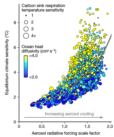
Source: Errickson et al. (2021)

Autocorrelation

Time series can also be auto-correlated, called an autoregressive model:

\[y_t = \sum_{i=1}^{t-1} \rho_i y_{t-i} + \varepsilon_t\]

Example: A time series is autocorrelated with lag 1 (called an AR(1) model) if \(y_t = \rho y_{t-1} + \varepsilon_t\).

Recap

Key Points

• Different model-relevant uncertainties (will matter later!)
• Reviewed probability distribution basics
  • Many different distributions, suitable for different purposes
  • Probability density functions vs. cumulative density functions

Key Points

• Frequentist vs. Bayesian probability (matters a bit later)
  • Frequentist: parameters as fixed (trying to recover with enough experiments)
  • Bayesian: parameters as random (probability reflects degree of consistency with observations)
  • In both cases data are random!

Key Points

• Confidence Intervals:
  • \(\alpha\)% of \(\alpha\)-CIs generated from different samples will contain the “true” parameter value
  • Do not say anything about probability of including true value!

Key Points

• Independence vs. Correlations
  • Do two variables increase/decrease together/in opposition or are they unrelated?
  • Can be very important scientifically!

References

Errickson, F. C., Keller, K., Collins, W. D., Srikrishnan, V., & Anthoff, D. (2021). Equity is more important for the social cost of methane than climate uncertainty. Nature, 592, 564–570. https://doi.org/10.1038/s41586-021-03386-6

Walker, W. E., Harremoës, P., Rotmans, J., Sluijs, J. P. van der, Asselt, M. B. A. van, Janssen, P., & Krayer von Krauss, M. P. (2003). Defining uncertainty: A conceptual basis for uncertainty management in model-based decision support. Integrated Assessment, 4, 5–17. https://doi.org/10.1076/iaij.4.1.5.16466